Annotating cell types with ginseng
In this tutorial, we provide a step-by-step guide on how to train a ginseng model, and how to use it to annotate new data. We will use single-cell RNA-seq data from human uterine tissue for this example.
Load data
The read_adata function from ginseng.data.io can be used to load 10x matrix market data, 10x h5 data, or in-memory or backed AnnData objects. In addition, as we show here, data can be downloaded and loaded directly by providing a URL endpoint.
from ginseng.data.io import read_adata

# Load uterine data from Ulrich et al. 2024
train = read_adata("https://datasets.cellxgene.cziscience.com/273ba93d-0751-4035-b1e1-d5c3a614beae.h5ad")

# Load uterine data from Tabula Sapiens
test = read_adata("https://datasets.cellxgene.cziscience.com/42f6f928-f6ef-41f5-9fed-4054027552d7.h5ad")
Preprocess data
Subset cell types
For simplicity, we will only train on cell types with more than 10 cells in both the training and test datasets. As ginseng takes raw counts as input, no preprocessing other than defining the subset of genes you wish to train on is necessary. For ease-of-use, ginseng provides a select_hvgs function that works on both in-memory and backed AnnData objects. If a backed object is provided, the HVGs are computed using a chunk-based strategy to avoid loading the entire dataset into memory.
# Count the number of cells per cell type in train and test
train_counts = train.obs.cell_type.value_counts().reset_index()
test_counts = test.obs.cell_type.value_counts().reset_index()

# Merge counts
merged_counts = train_counts.merge(
    test_counts,
    on="cell_type",
    how="outer",
    suffixes=("_train", "_test")
).fillna(0)

# Retain only cell types present in both datasets
merged_counts = merged_counts.loc[(merged_counts["count_train"] > 10) & (merged_counts["count_test"] > 10)]

# Subset train and test to only these cell types
train = train[train.obs.cell_type.isin(merged_counts["cell_type"])].copy()
test = test[test.obs.cell_type.isin(merged_counts["cell_type"])].copy()

# Store the raw counts
train.layers["counts"] = train.raw.X.copy()
test.layers["counts"] = test.raw.X.copy()
The final set of cell types we will be annotating in this tutorial.
| cell_type | count_train | count_test |
|---|---|---|
| B cell | 140 | 50 |
| ciliated epithelial cell | 4475 | 320 |
| fibroblast | 1585 | 6593 |
| macrophage | 3158 | 929 |
| mast cell | 882 | 65 |
| natural killer cell | 5356 | 92 |
Select highly variable genes
Now we can select the highly variable genes (HVGs) from the training dataset.
from ginseng.utils import select_hvgs

# Select highly variable genes (stored in train.var['ginseng_genes'])
select_hvgs(train, n_top_genes=2500, layer="counts")
[ginseng] Selecting genes: 100%|█████████████████████████████████████████████████████████████████████████████████████████████████████████████████████████████████████████████████| 4/4 [00:02<00:00, 1.76 chunks/s]
Construct a GinsengDataset
We can now setup a GinsengDataset which enables efficient data loading during training.
from ginseng.data import GinsengDataset

dataset = GinsengDataset.create("train.zarr", train, layer="counts", genes="ginseng_genes", label_key="cell_type")
[ginseng] Writing zarr: 100%|█████████████████████████████████████████████████████████████████████████████████████████████████████████████████████████████████████████████████████████| 4/4 [00:00<00:00, 8.37it/s]
If you didn't want to train the model now, you can retain the GinsengDataset on disk for later use, and re-load it as follows.
Train a classifier
For classification, all the required machinery for training a model is encapsulated in the GinsengClassifierTrainer class. This class takes care of setting up the model, optimizer, and data loaders, as well as the training loop itself. Below, we initialize a trainer using the dataset we created above.
from ginseng.train import GinsengClassifierTrainer, GinsengClassifierTrainerSettings

settings = GinsengClassifierTrainerSettings(
    # Augmentation parameters
    rate=0.1,
    lam_max=None,
    lower=0,
    upper=200,

    # Model parameters
    hidden_dim=64,
    dropout_rate=0.2,
    batch_size=128,

    # Training parameters
    lr=0.001,
    betas=(0.9, 0.999),
    eps=1e-8,
    weight_decay=0.01,
    normalize=True,
    target_sum=1e4,
    holdout_fraction=0.05,
    balance_train=True,
    group_level=False,
    group_mode="fraction",

    # Random seed for reproducibility
    seed=123
)

trainer = GinsengClassifierTrainer(dataset, settings)
Now we can train our model by calling the fit method on the trainer. The trained model and model state are returned after training is complete.
[ginseng] Epoch 1 report |  Training loss: 1.535e+00 | Holdout loss: 6.632e-01 | Holdout accuracy: 8.557e-01 |
[ginseng] Epoch 2 report |  Training loss: 4.782e-01 | Holdout loss: 3.550e-01 | Holdout accuracy: 9.483e-01 |
[ginseng] Epoch 3 report |  Training loss: 1.813e-01 | Holdout loss: 3.831e-01 | Holdout accuracy: 9.546e-01 |
[ginseng] Epoch 4 report |  Training loss: 1.747e-01 | Holdout loss: 2.428e-01 | Holdout accuracy: 9.572e-01 |
[ginseng] Epoch 5 report |  Training loss: 1.144e-01 | Holdout loss: 2.446e-01 | Holdout accuracy: 9.539e-01 |
[ginseng] Epoch 6 report |  Training loss: 5.886e-02 | Holdout loss: 2.288e-01 | Holdout accuracy: 9.516e-01 |
Annotate new data
If you are familiar with neural networks and jax, the model can be used to construct custom inference or training loops. However, for convenience, ginseng provides a simple API for annotating new datasets that only requires the model state. Assuming the same gene identifiers are present in the new dataset, annotation can be performed as follows.
Classify cells
UserWarning: Partial gene overlap detected: 99.92%.

[ginseng] Classifying: 100%|████████████████████████████████████████████████████████████████████████████████████████████████████████████████████████████████████████████████████████| 32/32 [00:00<00:00, 48.37it/s]
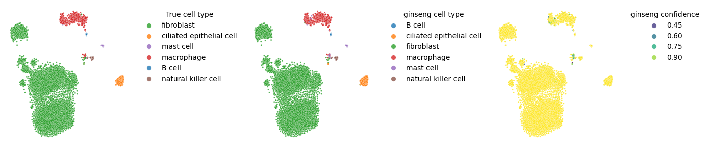
The predicted cell type labels from ginseng.classify can be found in the ginseng_cell_type column of the AnnData obs dataframe. Additionaly, the maximum predicted probability for each cell is stored in the ginseng_confidence column, which can be used to filter low-confidence predictions.
Note
Any time there isn't a perfect overlap between the genes used during training and a newly annotated dataset, ginseng will provide a warning specifying the fraction of overlapping genes. However, ginseng will automatically handle missing genes by inserting zero-valued columns for those genes during inference. To train a model robust to missing genes, it is recommended to use dropout on the input layer during training (rate > 0) and allow complete masking of genes during training (from lower to upper).
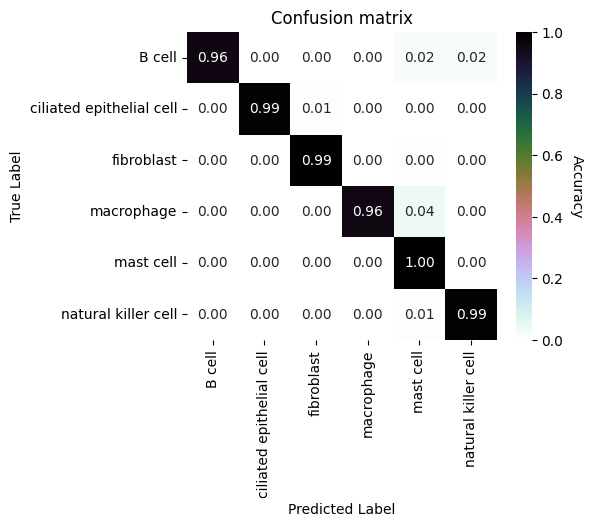
Evaluate performance
We will make a confusion matrix to visualize the performance of our classifier on the test dataset.
import pandas as pd
import seaborn as sns
import matplotlib.pyplot as plt

# Construct a confusion matrix
annotations = test.obs[["ginseng_cell_type", "cell_type"]].copy()
annotations["ginseng_cell_type"] = annotations["ginseng_cell_type"].astype(str)
annotations["cell_type"] = annotations["cell_type"].astype(str)
annotations['correct'] = annotations['ginseng_cell_type'] == annotations['cell_type']

confusion_matrix = pd.crosstab(
    annotations['cell_type'],
    annotations['ginseng_cell_type'],
    rownames=['True Label'],
    colnames=['Predicted Label'],
    normalize='index'
)

cell_types = merged_counts['cell_type'].tolist()
confusion_matrix = confusion_matrix.reindex(index=cell_types, columns=cell_types, fill_value=0)


fig, ax = plt.subplots(figsize=(5, 4))
sns.heatmap(confusion_matrix, annot=True, fmt=".2f", cmap="cubehelix_r", ax=ax)
cbar = ax.collections[0].colorbar
cbar.set_label('Accuracy', rotation=270, labelpad=15)
ax.set_title("Confusion matrix")
plt.show()
We will also visualize the true labels and predicted labels on an embedding for qualitative inspection.
import numpy as np
from sklearn.manifold import TSNE

# Normalize counts
X = test[:, test.var.index.isin(state.genes)].layers["counts"].toarray()
X = (1e4 * X.T / X.sum(axis=1)).T
X = np.log1p(X)

# Embedding
z = TSNE(n_components=2, random_state=123, perplexity=60.0).fit_transform(X)

# Plot annotated embeddings
fig, ax = plt.subplots(1, 3, figsize=(14, 3))

cell_type_palette = {k: v for k, v in zip(merged_counts['cell_type'], sns.color_palette('tab10', n_colors=len(merged_counts)))}

sns.scatterplot(
    x=z[:, 0], y=z[:, 1], hue=test.obs['cell_type'],
    palette=cell_type_palette, s=5, alpha=0.8, ax=ax[0]
)

sns.scatterplot(
    x=z[:, 0], y=z[:, 1], hue=test.obs['ginseng_cell_type'],
    palette=cell_type_palette, s=5, alpha=0.8, ax=ax[1]
)

sns.scatterplot(
    x=z[:, 0], y=z[:, 1], hue=test.obs['ginseng_confidence'],
    palette='viridis', s=5, alpha=0.8, ax=ax[2],
    hue_norm=(test.obs['ginseng_confidence'].min(), 1)
)

sns.move_legend(ax[0], "upper left", title="True cell type", frameon=False, bbox_to_anchor=(1.05, 1), markerscale=3)
sns.move_legend(ax[1], "upper left", title="ginseng cell type", frameon=False, bbox_to_anchor=(1.05, 1), markerscale=3)
sns.move_legend(ax[2], "upper left", title="ginseng confidence", frameon=False, bbox_to_anchor=(1.05, 1), markerscale=3)

for i in range(3):
    ax[i].axis('off')

fig.tight_layout()
Saving and loading models
ginseng models can be saved and loaded in a portable hdf5 format using the save_model and load_model functions. This allows you to save trained models to disk and load them later for inference or further training. For ease-of-use, the ginseng.classify function can perform classification directly from file paths pointing to the saved models and AnnData objects.